Research checkpoint #12: a DDoS attack against a more powerful machine
In post #10 from this series on my scientific initiation research, I discussed the results of simulating a DDoS attack against a Raspberry Pi 3B, trying to perform the packet sniffing on the live network traffic in the same way we were doing in the last experiments. Also, in the last post, I proposed a new step after the sniffing: to register the packets as CSV files, to further use them as a dataset for Machine Learning (ML) models. Advancing these studies, in this post I report a new simple experiment with simulated network traffic and performing an attack against a more powerful machine, trying to generate the CSV from this data to allow us to compare its performance with the Raspberry Pi.
Simulating network traffic with a more powerful machine
On this set of experiments, the client and server roles were inverted between the Raspberry Pi and the regular computer. The machines used for this set of experiments, connected in the same local network, are:
- Client:
- Intel(R) Core(TM) i7-6700K CPU @ 4.00GHz
- 32GB DDR4 2400 MHz RAM
- Debian GNU/Linux trixie/sid OS
- 1000 Mbits/sec network interface card (Gigabit Ethernet)
- Server: Raspberry Pi 3 Model B Plus Rev 1.3
- Quad Core 1.4GHz Broadcom BCM2837B0 64bit CPU
- 1GB RAM
- Raspbian GNU/Linux 10 (buster) OS
- 1000 Mbits/sec network interface card (Gigabit Ethernet)
The client used this Bash script to perform the experiments, five repetitions of each scenario, receiving the traffic from the server and trying to perform the conversion to CSV using the methods without an intermediary PCAP file that we studied in the last post. As the client was reporting the results through SSH, the numbers below may have a little additional volume because of this connection. Also, in addition to iperf3, I simulated a DDoS attack using the netwox tool. The traffic was configured to last for 10 seconds in both iperf3 and netwox, with additional time margins in the script to wait for the network to stabilize. The tools to collect the metrics are the same as those used in the last two posts. Below, I discuss each scenario.
Netwox with conversion to CSV using limited window
Trying to get to the limit of our sniffing script, in this experiment I performed the CSV generation without the intermediary PCAP using a window of size 10 and a buffer with 20000 positions, similar to the most performatic configuration we found in our previous experiments, but with adjusts in the buffer size, as now the traffic considered is the flood generated by netwox. The duration of the attacks were the same. The metrics collected are:
| Metric | Mean | Standard Deviation | Min | Max |
|---|---|---|---|---|
| CPU usage | 67.6% | 5.09% | 60.9% | 74.9% |
| Memory usage | 168995.2KB | 2284.53KB | 166244KB | 172340KB |
| Duration of execution | 52.905s | 0.503s | 52.495s | 53.698s |
| Number of lines in final CSV file | 8308.2 | 706.98 | 7358 | 9181 |
Considering that each line of the final CSV file corresponds to 10 packets analysed, the amount of packets processed here isn’t so distant from the number registered in post #10 by the duo Pypcap + dpkt, a gain of only ~13%, as can be seen in comparison in the graph below. However, it is notable that the standard deviation is much more significant in this case, indicating a great variation in the values over the five executions. Even so, the minimum number of packets counted was 73580 (7358 lines in CSV), a number still bigger than the mean observed in the previous experiments. The library used to sniff the packets in this experiment is again Pypcap and the scripts to generate the CSV use dpkt.
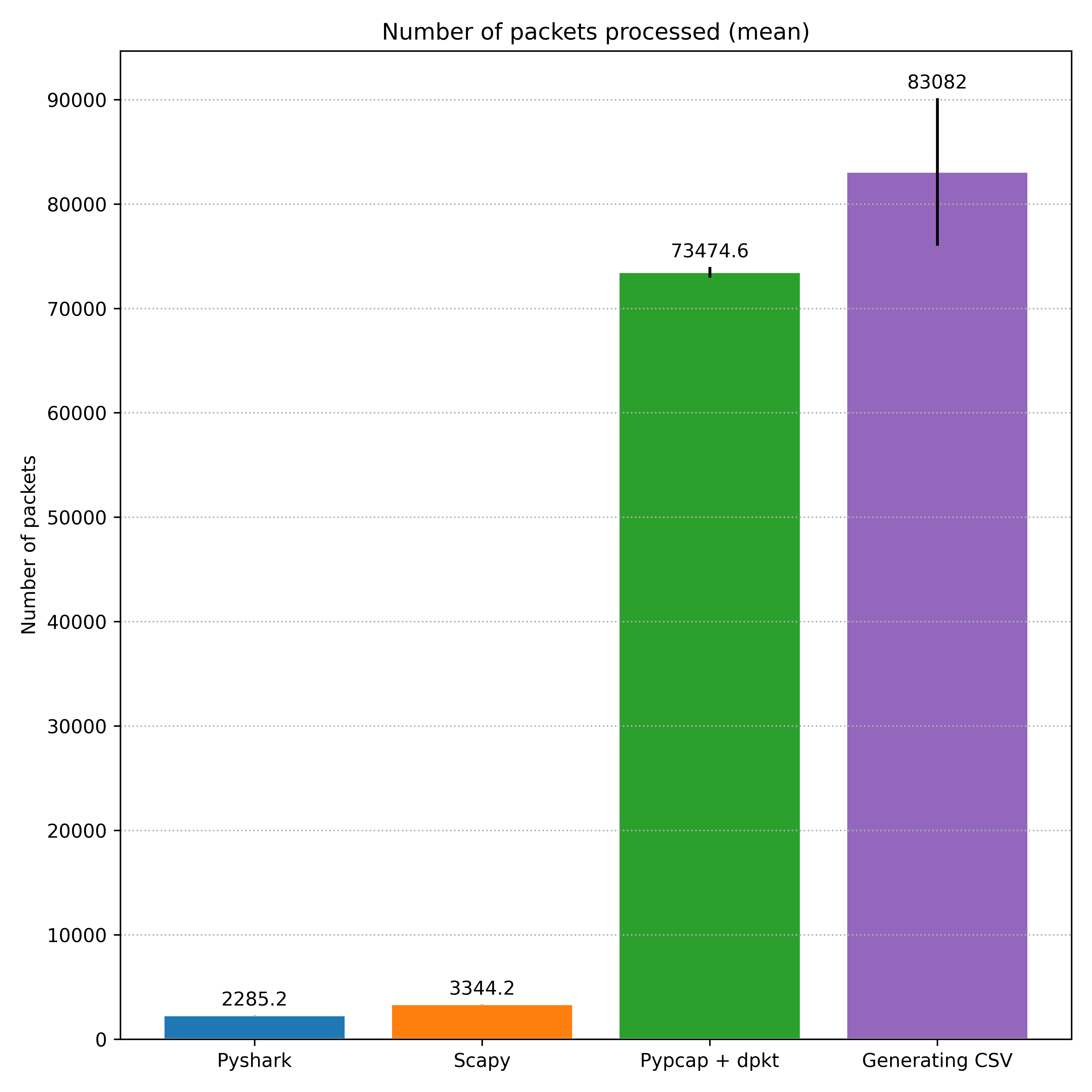 Number of packets processed by the libraries in post 10 compared with the one in our experiment here.
I don’t have the exact number of packets produced by the netwox tool, as it doesn’t do a report, but empirically I estimated that it is something around 120.000. The adjustment to the buffer size was considering this number, to be able to possibly store all the packets simultaneously. However, even with a better computer, we’re still losing a lot of packets in the final count: if my estimates are correct, around 30% of all the traffic is not counted.
The duration of the execution is coherent with what we expect, as there was a gap of 10 seconds before and 30 seconds after the traffic, totaling something close to 50 seconds. The metrics of performance are also good, with controlled CPU usage and memory. Notice that it is not possible to compare the usage of CPU observed here to the one in post 10, as here we are now processing the packets more intensively after the sniffing process. The same applies to the memory consumption, it’s expected to have bigger values here.
Iperf3, 25Mbits/s UDP
As we are dealing with a more powerful computer processing the packets compared to the Raspberry Pi we were using, a natural question that arises is how it will deal with the same set of experiments we did in the last post. For comparison, I performed only the executions with 25Mbits/s of bit rate, using the same process as described here. The results are as follows.
- With limited window of 10 packets (window of size 10 and buffer with 5000 positions):
| Metric | Mean | Standard Deviation | Min | Max |
|---|---|---|---|---|
| CPU usage | 25.82% | 1.58% | 24.1% | 27.6% |
| Memory usage | 171639KB | 211.44KB | 171412KB | 171968KB |
| Duration of execution | 37.021s | 2.83s | 34.205s | 40.259s |
| Number of lines in final CSV file | 2231 | 10.77 | 2212 | 2238 |
- With unlimited window (window of size 50000 and buffer with 10 positions):
| Metric | Mean | Standard Deviation | Min | Max |
|---|---|---|---|---|
| CPU usage | 62.72% | 2.06% | 59.1% | 64.0% |
| Memory usage | 272117.6KB | 1042.88KB | 271064KB | 273708KB |
| Duration of execution | 1m32.05s | 2.42s | 1m30.315s | 1m36.215s |
| Number of lines in final CSV file | 2281 | 24.04 | 2249 | 2315 |
Considering that the total number of packets produced by iperf3 was 21584 in the transmission stream and that each line of the CSV represents 10 packets (except for the last one, which is the remainder), the loss here is zero! We have more packets than expected because this data was collected using an SSH connection, so there is another traffic in the network. But it is very interesting to see the impact that the computational capacity had on the result: we didn’t lose packets using the first scenario with only 37s on average, a way better than the 5m40s of average found using the intermediary PCAP in our experiments from the last post.
Comparing the obtained numbers with the ones in the same scenarios from the last post, we can see that we had a huge improvement: with limited window of 10 packets, here our average use of CPU was 25.82%, and there it was 81.40%; the same applies with the unlimited window, here we had 62.72% and there 96.62%. The most impressive number in this last case is the time of execution: here we only had 1m32s, there the average was 16m29s, and with a lower CPU usage. Very interesting! The memory usage, on another hand, isn’t so discrepant, presenting a bigger value here.
Concluding, the hardware improvement has a great impact on the numbers observed. This is not a surprise, but confirms our intuitions. The challenge is how to use the most of the hardware we have, even operating on low performance computers, to always achieve good results.
About a new tool: hping3
So far, we have been using netwox to generate DDoS attack simulations. Another interesting tool we discovered that can be used for this function is hping3. This tool provides a lot of functionalities, from just working as the regular ping command to sending custom TCP/IP packets. Some interesting options can be used to simulate a DDoS attack:
--rand-source: uses random IP addresses as source for the packets.--rand-dest: uses random IP addresses as destination for the packets. Permits also to use a mask to determine which field of the IP to randomize (e.g., ‘10.0.0.x’ will randomize only the last field of the IPv4).--data: can be used to adjust the packet body size.--interval: can be used to set the number of seconds or microseconds between each packet in the transmission.--flood: send the packets as fast as possible, can be used to try to flood the target.
Many other options are listed in its manual page, these are just some of the ones I found to be most interesting.
Submissions to events
In the last blog post, I mentioned that me and professor Daniel submitted papers to two events in our field of study, the WTG (Workshop on Undergraduate and Scientific Initiation Works, part of the 43º Brazilian Symposium on Computer Networks and Distributed Systems) and WPerformance (Workshop on Performance of Computing and Communication Systems, part of the 45º Brazilian Computer Society Congress). Both of them were accepted! You can find the complete articles in the links below:
- SILVA, Otávio O.; BATISTA, Daniel M.. Adequação Online de Rastros de Tráfego de Rede nos Clientes para Alimentar Sistemas de Detecção de Intrusão. In: WORKSHOP DE TRABALHOS DE INICIAÇÃO CIENTÍFICA E DE GRADUAÇÃO - SIMPÓSIO BRASILEIRO DE REDES DE COMPUTADORES E SISTEMAS DISTRIBUÍDOS (SBRC), 43. , 2025, Natal/RN.
- SILVA, Otávio O.; BATISTA, Daniel M.. Performance Evaluation of Python Tools to Capture Packets in Resource-Constrained Devices. In: WORKSHOP ON PERFORMANCE OF COMPUTER AND COMMUNICATION SYSTEMS (WPERFORMANCE), 24. , 2025, Maceió/AL.
Next steps
Including the work in this post, our current goal is to determine the best experimentation environment and to understand its limitations. Observing these results, our next steps will be on joining the packet sniffing with AI models to perform the inference of live network traffic, understanding the process of connecting these ends and performing an initial analysis of the performance we can expect from doing both the sniffing and inference together. So, our current plans are:
- Packet Parsing
- Conduct experiments to verify the performance of Python libraries sniffing the network and processing the packages in a Raspberry Pi (different from what we did in post 4, in which we tested the lib’s with the CIC-IoT-2023 dataset and in a regular computer).
- [NEW] Study mechanisms for generating CSV files from PCAP ones or directly from live network traffic.
- Inference
- Run the baseline models proposed in post 02 in a Raspberry Pi to verify its performance.
- Perform experiments connecting the packet sniffer to the AI baseline models.
- Training (centralized IDS)
- TBD.
This post was made as a record of the progress of the research project “DDoS Detection in the Internet of Things using Machine Learning Methods with Retraining”, supervised by professor Daniel Batista, BCC - IME - USP. Project supported by the São Paulo Research Foundation (FAPESP), process nº 2024/10240-3. The opinions, hypothesis and conclusions or recommendations expressed in this material are those of the author and do not necessarily reflect the views of FAPESP.