Research checkpoint #14: dimensionality reduction of the CIC-IoT-2023
In the last two posts, we have been conducting experiments in a more powerful machine to understand and compare its results with our observations with the Raspberry Pi, our target device in this project, as we are evaluating how low-performance computers can handle different steps of an Intrusion Detection System (IDS) based on machine learning models. In particular, in the last post we discussed the performance of this powerful machine using the baseline models we presented in post #06, namely the Logistic Regression and the Hoeffding Tree models. One debt from this older post that we have, however, is that the Raspberry Pi was unable to run these models with the CIC-IoT-2023 dataset due to memory limitations. In this post, we attack this problem! Here, we expect to understand more clearly the limitations of this device in executing the entire training and inference process with ML models, placing a different emphasis from our studies on the sniffing phase.
One of the first subjects we studied in this research project was feature engineering, as highlighted in post #01, and two topics are especially interesting for our current context: Mutual Information and Principal Component Analysis (PCA). Both of them, the first one a metric that can be used to quantify how one feature impacts the label and the second a technique to capture the largest variations in the data, can be used to reduce the dimension of the dataset. In this way, we can reduce the memory requirements to handle the data and give hope for the Raspberry Pi to process it, while trying not to lose much information. In the sections below, we explore more about these two topics of interest.
Mutual Information
Mutual Information is a measure of how the knowledge of one random variable can reduce the uncertainty about other one, being very useful in the context of feature selection: the idea is to compute how each feature from our dataset impacts the label and, then, work only with the ones that have the biggest influence. In this way, our expectations are to discard the values that don’t contribute much to our classification of the network traffic as malicious or benign. The scikit-learn library has an easy-to-use implementation of this metric, all the scripts utilized for this end can be found here.
The CIC-IoT-2023 have 39 features in total, a full list with details on each one can be found on their website. After computing the mutual information of each one with the label without previously scaling the data, working with the first four files of the final CSVs generated by the authors (586MB in total), this is our top-10:
| Feature | M.I. with label |
|---|---|
| Time_To_Live | 0.273604 |
| IPv | 0.271849 |
| LLC | 0.271835 |
| Header_Length | 0.204124 |
| AVG | 0.188707 |
| Tot size | 0.188701 |
| TCP | 0.157581 |
| Tot sum | 0.079654 |
| Number | 0.076874 |
| UDP | 0.072344 |
The bigger the values, the better. Observing numbers that aren’t so expressive can be an indication that the features may not be directly associated with our classification individually, so it is reasonable to select the ones that produce the highest results. After some preliminary experiments, I decided to set a threshold of 0.20 to keep the features, selecting just the first four ones in the rank. Considering the table, it is a high cut value and we are discarding significant information, but our main goal here is to reduce the amount of data we are working on, and this threshold has shown to be a good choice for this purpose, resulting in a final file with 98MB.
This final file obtained was utilized to train a Hoeffding Tree model, using an online approach: the model tries to infer each entry of the dataset and, then, learn with it, as we are working with labeled data. The script used for this can be found here. This script was run 10 times, registering the total time spent and the peak of memory during each iteration on two different computers:
- Raspberry Pi Model 3 B
- Quad Core 1.2GHz Broadcom BCM2837 64bit CPU
- 1GB RAM
- Debian GNU/Linux 12 (bookworm) OS
- 100 Mbits/sec network interface card (Fast Ethernet)
- Reference computer
- Intel(R) Core(TM) i7-6700K CPU @ 4.00GHz
- 32GB DDR4 2400 MHz RAM
- Debian GNU/Linux trixie/sid OS
- 1000 Mbits/sec network interface card (Gigabit Ethernet)
The values observed were:
| Device | Average time | Peak of memory use |
|---|---|---|
| Raspberry Pi | 53m48.263s | 615312KB (~615MB) |
| Reference computer | 4m30.409s | 626880KB (~627MB) |
The reference computer had a reduction of plus than 90% in the average time of execution compared with the Raspberry Pi, both with a low standard variance (close to 1%). However, besides this disparity, it is already great to observe that the low-performing computer was able to run the model! Even using a few megabytes less than the reference. Still regarding the memory, remember that our CSV file used here has 98MB, and our peak here was almost 627MB, a huge increase, almost 540%. We will discuss this in a section below when we compare these metrics with the ones we achieved with the original dataset; for now, our principal observation is the difference in performance in terms of execution time: the difference in hardware is very impactful.
The accuracy achieved by the model in this scenario was 98.26%, and considering that our dataset has 2834737 entries, we made a mistake only in around 50000 entries. At first glance, this sounds amazing; however, our support is very unbalanced: we are classifying the network traffic as benign and malicious, but only 2.3% of it is benign, that is, 66392 entries. If we classify all the data as malicious, we would still have an accuracy of 97.7%, a very misleading number. We already pointed this out in post #06, a problem that makes it difficult for us to evaluate this technique in terms of its effectiveness, just by observing this number.
We can look at other metrics: for the benign label, we got a recall of 56.37%. Considering that this value represents the percentage of the actual benign entries the model was able to correctly identify, its performance was a little above a coin toss. It is not completely random, but still far from what we would like in a real-world scenario, as the majority of network traffic we would see in a network probably is benign on a normal day. The precision (percentage of traffic classified as benign that is actually benign) observed was 64.72%, a bit better, but also far from being a good number, with a lot of false positives. Therefore, we achieved our goal of reducing the dimensionality of the model, but at a great cost in terms of effectiveness.
Principal Components Analysis (PCA)
Similarly to what we have done in the last section with the mutual information metric, the idea here is to use PCA to also reduce the dimensionality of the dataset, in this case using feature projection. The Principal Component Analysis is a technique that finds the axes of the greatest variation of data and then, through a linear transformation, projects the entries on this new basis. In this way, considering each entry as a point in this new coordinate system, it becomes easier to better understand the data, identifying the directions of its greatest variations. Note that, different from the last approach, here we are not looking at the label feature, just at the normal features themselves, observing their behavior. The implementation of this technique used was also the one from scikit-learn, code available here.
As pointed out before, our dataset has 39 different features, that is, 39 dimensions. Running the PCA on it returns a new basis, with the projections of each entry from the original dataset on it. The axes are ordered by their variance, and we can compute the contribution of each of them to the total variance of the data (explained_variance_ratio_ parameter). Here are the 15 with highest contribution:
| Feature | Explained variance |
|---|---|
| 1 | 14.28% |
| 2 | 11.44% |
| 3 | 9.75% |
| 4 | 7.77% |
| 5 | 7.03% |
| 6 | 4.96% |
| 7 | 4.50% |
| 8 | 4.26% |
| 9 | 3.46% |
| 10 | 3.03% |
| 11 | 2.63% |
| 12 | 2.56% |
| 13 | 2.55% |
| 14 | 2.53% |
| 15 | 2.51% |
For our experiments, I decided to work with all the features that have a contribution bigger than 3%, that is, the first 10 features from the table above, explaining around 70.5% of the total variance in the data. The final CSV file containing only these features has 609MB, but despite this large number, surprisingly, the peak of memory use over 10 repetitions of the experiment with the Hoeffding Tree model was not so distant from what we observed also with the mutual information best features:
| Device | Average time | Peak of memory use |
|---|---|---|
| Raspberry Pi | 1h17m11.692s | 661596KB (~662MB) |
| Reference computer | 6m6.386s | 679928KB (~680MB) |
If in the peak of the last section we consumed 627MB, here our peak was 680MB, a difference of only 53MB. Considering that the file here is 521% bigger than the one we achieved with M.I., this is a huge difference. It is not clear to me the reason for that, maybe the model was more suitable for this representation of the data (after the PCA), given that the model is the unique constant over the experiments. On another hand, if we didn’t have an expressive difference in memory, in the average time of execution the difference was more expressive: here, we consumed more than 20 minutes more than in the scenario with M.I. using the Raspberry Pi. Proportionally, the results here were almost the same as the last section, as the reference computer reduced by plus than 90% the average time of execution, coherent.
However, again the unbalancing of the data was a problem, a little better than with the M.I. technique, but still with a performance under what we would like for an IDS: we achieved 98.55% of accuracy, but 65.75% of recall and 70.41% of precision for the benign label. We had an improvement here, and as PCA don’t evaluate the features individually like M.I., this may be an indication that we can extract util information by observing groups of them and studying the numbers together.
Comparing with the original experiment
Using the data from the last post, in which we ran the Hoeffding Tree model with the CIC-IoT-2023 dataset on our most powerful machine (the reference computer here), we can compare the results obtained:
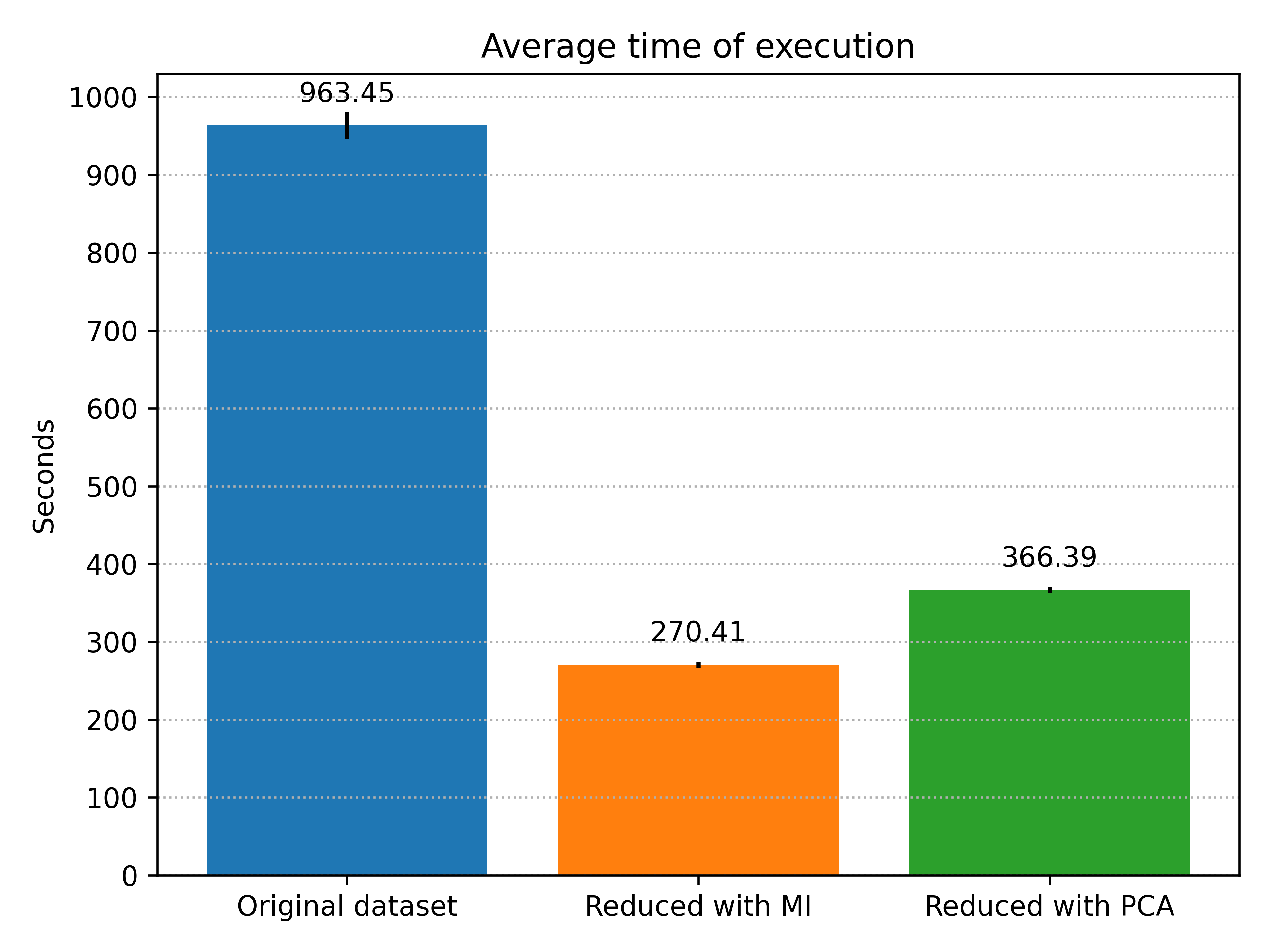
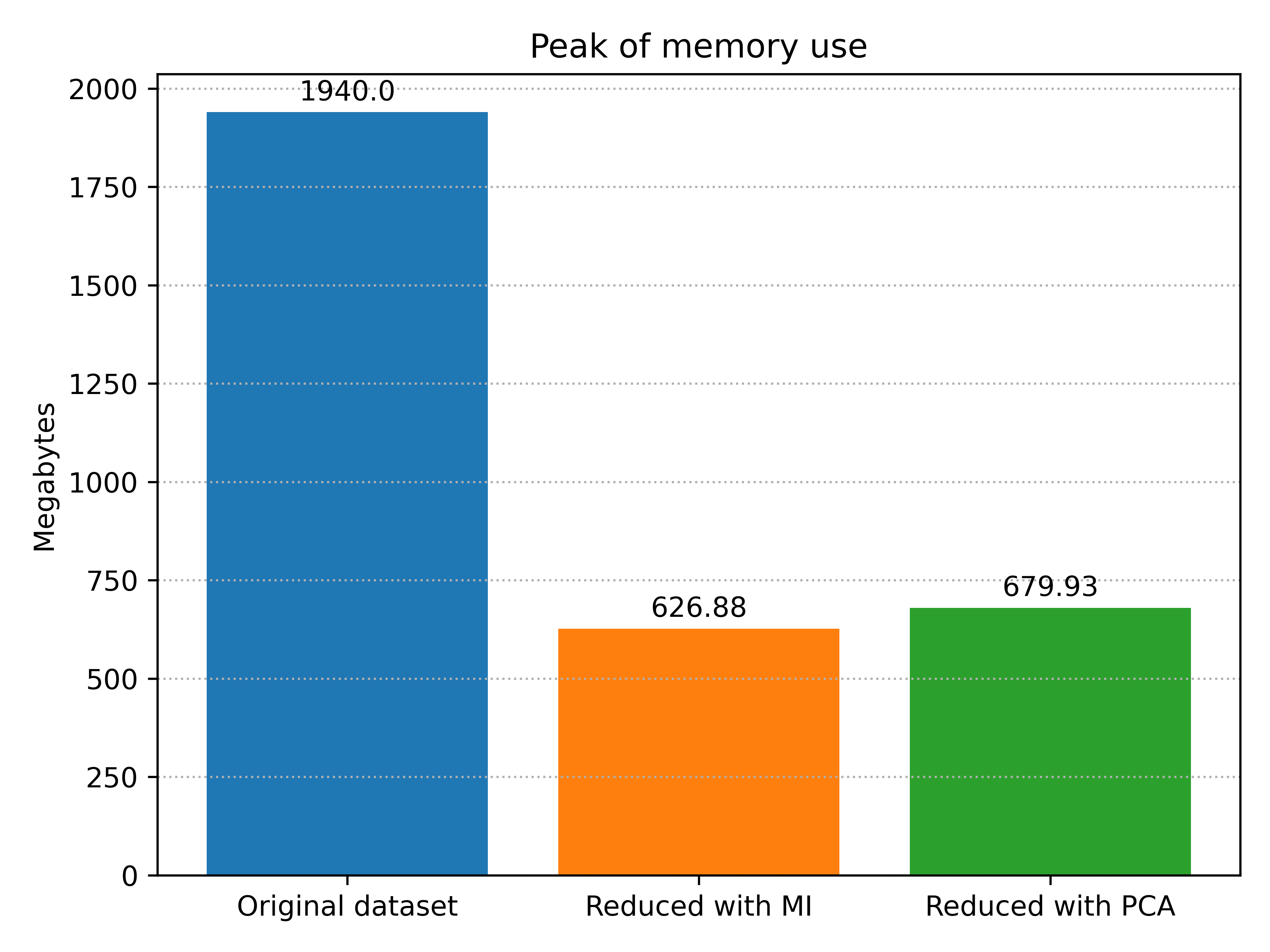
The first thing that can catch your attention is how close the two experiments with reduced dataset are, considering that with one we have 4 features (M.I.) and with the other 10 (PCA), especially observing the memory. As discussed in the last section, it is not clear to me the reason for that, but still interesting. But we achieved our goal: the memory had a significant reduction and the execution time also, permitting the Raspberry Pi to execute the model without wasting all of its resources.
For comparison, we achieved 98.73% of accuracy with the original dataset, a value very close to the ones we observed above. For the other metrics, we achieved 75.49% of recall and 71.85% of precision. They are better than the ones we observed before, but considering that here we have all of our data in its original form (or, at least, the first four files of the dataset), they could be even better, especially considering the criticality of network traffic classification.
Next steps
After these experiments, we have a better understanding of the expected computational performance of a hardware-limited device dealing with network traffic data and ML models, even without much to discuss about the impacts on accuracy with the techniques considered. Focusing on this performance analysis, we saw that the improvement on hardware had a meaningful impact, but it is not clear if this is something that affects the whole process: we are performing both the training and inference, are both of them being significantly affected? Our next step will be in this direction, performing only the inference on the Raspberry Pi and the model training on a central machine, understanding if this leads to gains for the low-performance computer. We already proposed this in last post, the idea of distributed inference, we will discuss it in the next post.
This post was made as a record of the progress of the research project “DDoS Detection in the Internet of Things using Machine Learning Methods with Retraining”, supervised by professor Daniel Batista, BCC - IME - USP. Project supported by the São Paulo Research Foundation (FAPESP), process nº 2024/10240-3. The opinions, hypothesis and conclusions or recommendations expressed in this material are those of the author and do not necessarily reflect the views of FAPESP.