M2 research ckpt #01: multiplying agents

Posted Nov 6, 2026

By Otávio de Oliveira Silva

14 min read

During this last month, I have been laying my foundations in Reinforcement Learning. In the previous and first checkpoint, I had established the basis in Single-Agent RL. Now, on top of it, I advanced to the next natural step: Multi-Agent RL. In this checkpoint, I present what I have studied so far and also conclude with my presentation notes on a paper that proposes an extension of the TRPO/PPO algorithms to the multi-agent setting.

So far

To explore the multi-agent setting of machine learning, my main resources were the following chapters of the “Multi-Agent Reinforcement Learning: Foundations and Modern Approaches” book¹:

Chapters 3 (“Games: Models of Multi-Agent Interaction”) and 4 (“Solution Concepts for Games”): These chapters introduce the dynamics behind the interaction of agents in an environment through Game Theory, providing an overview of the models of multi-agent interaction (Normal-Form Games, Repeated Normal-Form Games, Stochastic Games, and Partially Observable Stochastic Games) and solution concepts (Minimax, Nash Equilibrium, $\epsilon$-Nash Equilibrium, and Correlated Equilibrium). It also discusses some limitations of these equilibrium solutions and possible additional criteria (Pareto Optimality, Welfare Optimality, Fairness Optimality, and No-Regret).
Chapters 5 (“Multi-Agent Reinforcement Learning in Games: First Steps and Challenges”) and 6 (“Multi-Agent Reinforcement Learning: Foundational Algorithms”): Given the theory, throughout these chapters we see the application of RL to games. The approaches go from simple Central and Independent Learning to more advanced ones, covering Value Iteration, Joint-Action Learning, Agent Modeling, and Policy-Based Learning.
Chapter 9 (“Multi-Agent Deep Reinforcement Learning”): Finally, here we extend RL algorithms by using Deep Learning. Under the Centralized Training and Decentralized Execution (CTDE) paradigm, the chapter proposes Multi-Agent Policy Gradient algorithms, Value Decomposition, and an extension of Agent Modeling to the multi-agent setting. It also discusses how the approach differs when agents are homogeneous.

Paper presentation: TRPO in MARL

To consolidate all these concepts seen during the last few weeks, I was tasked with presenting the paper “Trust Region Policy Optimisation in Multi-Agent Reinforcement Learning” by J. G. Kuba et al.² to my classmates in the Master in Cybersecurity. This work introduces an extension of the trust region methods proposed in single-agent RL to the multi-agent context, while keeping the monotonic performance improvement guarantee. In this section, I write down my presentation notes, trying to give the intuition behind the paper in ~20 minutes, quite a challenge.

Context and motivation

Machine learning is usually decomposed into three big paradigms: supervised learning, unsupervised learning, and reinforcement learning (RL). This last one, particularly, has gained traction in the cybersecurity field, since agents trained under this paradigm can be highly flexible to changes in the environment, without human intervention or labeled data, which is great against attack scenarios.

You probably have heard some recent examples of applications of RL in the cybersecurity field, for example, the Hugging Face incident³. In summary: OpenAI’s agents being trained using the RL paradigm against a cybersecurity task were able to break through their “air-gapped” sandbox and reach the internet, where they promoted a data exfiltration attack against Hugging Face, trying to search for clues to solve their task.

This wasn’t the only recent case that we know about. Anthropic’s model Claude Mythos, with strong capabilities in cybersecurity, is being used in a closed verification program to find zero-day vulnerabilities in many major software systems. It has not been released to the general public due to risk concerns.

Therefore, RL is highly relevant in the cybersecurity field, for both defenders and attackers. Here, I’ll give a brief introduction to how it works under the hood and scale from single-agent to multi-agent scenarios, presenting a relevant algorithm and its extension to environments with multiple agents.

Preliminaries

Brief introduction to RL and notation

Reinforcement learning algorithms learn solutions for sequential decision processes via repeated interactions with an environment. This can be modeled as a Markov game, composed of:

A set of agents, $\mathcal{N} = \{1, \dots, n\}$;
A finite state space $\mathcal{S}$;
A joint-action space $\mathcal{A} = \prod_{i=1}^n \mathcal{A}^i$, the product of finite action spaces $\mathcal{A}^i$ of each agent $i \in \mathcal{N}$;
A transition probability function between states, $\mathcal{P} : \mathcal{S} \times \mathcal{A} \times \mathcal{S} \rightarrow [0,1]$; and
A reward function $r : \mathcal{S} \times \mathcal{A} \rightarrow \mathbb{R}$.

At time step $t \in \mathbb{N}$, each agent $i \in \mathcal{N}$ observes the current state $s_t \in \mathcal{S}$ and takes an action $a^i_t \in \mathcal{A}^i$ drawn from its policy $\pi^i(\cdot \vert{} s_t)$, a probability distribution over its action space given the current state. This is done simultaneously across agents, which together form a joint action $a_t = (a_t^1, \dots, a_t^n)$, sampled from a joint policy $\pi(\cdot \vert{} s_t) = \prod_{i=1}^n \pi^i(\cdot^i \vert{} s_t)$. Given the joint action, the environment is then moved to the state $s_{t+1} \in \mathcal{S}$ with probability $\mathcal{P}(s_{t+1} \vert{} s_t, a_t)$.

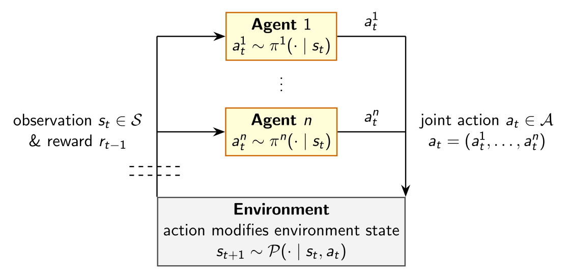Basic loop for $n$ agents interacting with an environment.
Image create with the help of Gemini, inspired on Figure 2.2 of the MARL book¹.

We’ll assume a fully cooperative setting, where all agents share the same common reward function. Once the agents choose a joint action at time $t$ they receive a reward $r_t$. Their goal is to maximize the expected total reward, given a discount factor $\gamma \in [0, 1)$:

\[J(\pi) = \mathbb{E}_{\pi} \left[ \sum_{t=0}^\infty \gamma^t r_t \right]\]

Three important functions to keep in mind:

Function name	Equation	Intuition
State value	$V_{\pi}(s) = \mathbb{E}_{\pi} [ \sum_{t=0}^\infty \gamma^t r_t \vert{} s_0 = s ]$	What is the expected total reward starting on state $s$ and following $\pi$?
State-action value	$Q_{\pi}(s, a) = \mathbb{E}_{\pi}[ \sum_{t=0}^\infty \gamma^t r_t \vert{} s_0 = s, a_0 = a ]$	What is the expected total reward starting on state $s$, taking specific action $a$, and then following $\pi$?
Advantage	$A_{\pi}(s, a) = Q_{\pi}(s, a) - V_{\pi}(s)$	How much better is action $a$ than the average behavior in state $s$?

These functions can also be extended to subsets of agents. Let $i_{1:m}$ denote an ordered subset $\{i_1, \dots, i_m\}$ of $\mathcal{N}$, and let $-i_{1:m}$ denote its complement. The multi-agent state-action value function is defined as:

\[Q_{\pi}^{i_{1:m}}(s, a^{i_{1:m}}) = \mathbb{E}_{a^{-i_{1:m}} \sim \pi^{-i_{1:m}}} \left[ Q_{\pi}(s, a^{i_{1:m}}, a^{-i_{1:m}}) \right]\]

For disjoint sets $j_{1:k}$ and $i_{1:m}$, the multi-agent advantage function is:

\[A_{\pi}^{i_{1:m}}(s, a^{j_{1:k}}, a^{i_{1:m}}) = Q_{\pi}^{j_{1:k}, i_{1:m}}(s, a^{j_{1:k}}, a^{i_{1:m}}) - Q_{\pi}^{j_{1:k}}(s, a^{j_{1:k}})\]

The idea is: how much better are actions $a^{i_{1:m}}$, assuming agents $j_{1:k}$ have already locked in their new strategies?

TRPO and PPO

The Trust Region Policy Optimization (TRPO) algorithm⁴ was proposed in the single-agent RL context, and has the amazing property of guaranteeing a monotonic improvement of $J(\pi)$ at each iteration. In practice, given a parametrized policy $\pi_\theta$ (for example, a neural network with parameters $\theta$), the TRPO update at iteration $k+1$ is given by:

\[\theta_{k+1} = \underset{\theta}{\text{argmax }} L_{\pi_{\theta_k}}^{TRPO}(\pi_\theta), \text{ subject to } \mathbb{E}[D_{KL}(\pi_{\theta_k}, \pi_{\theta})] \le \delta\]

, where $L_{\pi_{\theta_k}}^{TRPO}(\pi_\theta) = \mathbb{E}_{s \sim \mathbb{P}(\cdot \vert{} \pi_{\theta_k}), a \sim \pi_{\theta}} \left[ A_{\pi_{\theta_k}}(s, a) \right]$ is the “loss function” associated with the policies, and $D_{KL}$ is the Kullback–Leibler divergence, which can be thought of as a measure of distance between the two probability distributions. Hence, we update the old policy to a new one that is, at most, at a distance of a constant $\delta$, moving in the direction that maximizes the advantage in the current environment within the trust region.

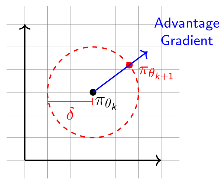A visualization of the improvement from $\pi_{\theta_k}$ to $\pi_{\theta_{k+1}}$.
Image created with the help of Gemini.

However, dealing with the divergence term has high computational costs. The Proximal Policy Optimization (PPO) algorithm⁵ is proposed as an approximation to TRPO that reduces this cost by dropping the constraint and maximizing the following objective:

\[L^{\text{PPO}}_{\pi_{\theta_k}}(\pi_\theta) = \mathbb{E}_{s \sim \mathbb{P}(\cdot \vert{} \pi_{\theta_k}), a \sim \pi_{\theta_k}} \left[\min \left( \frac{\pi_\theta(a \vert{} s)}{\pi_{\theta_k}(a \vert{} s)} A_{\pi_{\theta_k}}(s, a), \text{ clip} \left(\frac{\pi_\theta(a \vert{} s)}{\pi_{\theta_k}(a \vert{} s)} , 1 \pm \epsilon \right) A_{\pi_{\theta_k}}(s, a) \right) \right]\]

Note that here the action is sampled from the policy $\pi_{\theta_k}$ from the previous iteration, not the new candidate $\pi_\theta$ as in the TRPO loss. The ratio $\frac{\pi_\theta(a \vert{} s)}{\pi_{\theta_k}(a \vert{} s)}$, called “importance weight”, is what allows us to use data from the old policy to learn the new one. The clip operator replaces this term with $1+\epsilon$ or $1-\epsilon$ depending on whether it is beyond the threshold interval and, in this way, PPO controls the size of policy updates. Intuitively, the logic is the same: “the new policy does not benefit by going far away from the old policy”, as explained in OpenAI Spinning Up docs⁵.

Multiplying Agents

Given these algorithms for the single-agent scenario, extending the methods to the multi-agent setting is not a simple task. One naive approach, for example, would be to endow each agent with its own parameters and run the algorithm independently. Although the reward functions increase in each of the agents’ update directions, it isn’t guaranteed that the global outcome will improve monotonically. In fact, it can get worse.

Extending TRPO and PPO to multiple agents

Assuming that all the policies are $\eta$-soft⁶, the key lemma to extend the previous ideas to the multi-agent scenario is the following one:

Lemma 1 (Multi-Agent Advantage Decomposition): In any cooperative Markov game, given a joint policy $\pi$, for any state $s$, and any agent subset $i_{1:m}$, the following equation holds.
\[A_\pi^{i_{1:m}}(s, a^{i_{1:m}}) = \sum_{j=1}^m A_\pi^{i_j}(s, a^{i_{1:j-1}}, a^{i_j})\]

Intuitively, the joint advantage function can be decomposed into a sum of each agent’s local advantages, and we can compute agent’s $i_j$ local advantage given its own action and the ones from agents $\{i_1, \dots, i_{j-1}\}$.

This suggests an approach: let agents take actions sequentially, following an arbitrary order $i_{1:m}$, assuming agent $i_1$ takes action $a^{i_1}$ such that $A^{i_1}(s, a^{i_1}) > 0$, and then, for $m=2, \dots, n$, agent $i_m$ takes an action $a^{i_m}$ such that $A^{i_m}(s, a^{i_{1:m-1}}, a^{i_m}) > 0$. The lemma assures us that the final advantage $A_{\pi_\theta}(s, a)$ will be positive and, consequently, we can improve the performance.

What the Heterogeneous-Agent Trust Region Policy Optimisation (HATRPO) algorithm proposes in practice is to, at every iteration $k+1$, given a permutation⁷ $i_{1:n}$, optimize the policy parameter $\theta_{k+1}^{i_m}$ for every agent $i_{m \in \{1, \dots, n\}}$ in sequence by maximizing the constrained objective:

\[\theta_{k+1}^{i_m} = \underset{\theta^{i_m}}{\text{argmax }} \mathbb{E}_{s \sim \mathbb{P}(\cdot \vert{} \pi_{\theta_k}), \text{ } a^{i_{1:m-1}} \sim \pi_{\theta_{k+1}^{i_{1:m-1}}}^{i_{1:m-1}}, \text{ } a^{i_m} \sim \pi_{\theta^{i_m}}^{i_m}} \left[ A_{\pi_{\theta_k}}^{i_m}(s, a^{i_{1:m-1}}, a^{i_m}) \right],\\ \ \\ \text{ subject to } \mathbb{E}[D_{KL}(\pi_{\theta_k^{i_m}}^{i_m}, \pi_{\theta^{i_m}}^{i_m})] \le \delta\]

This algorithm enjoys the monotonic improvement property in the same way as TRPO for the single-agent setting, as demonstrated in Section 3.2 of the original paper² with a non-parametrized theoretical version of the algorithm. A closed-form update can be obtained by applying some approximations.

A challenge persists: we still need to handle individual advantage functions for each agent, with inputs varying in size since the permutation doesn’t need to be the same across iterations. The trick proposed by the authors is to use Lemma 1 to rewrite this expectation:

Proposition 2: Let $\pi = \Pi_{j=1}^n \pi^{i_j}$ be a joint policy, and $A_\pi(s,a)$ be its joint advantage function. Let $\bar{\pi}^{i_{1:m-1}} = \Pi_{j=1}^{m-1} \bar{\pi}^{i_j}$ be some other joint policy of agents $i_{1:m-1}$, and $\hat{\pi}^{i_m}$ be some other policy of agent $i_m$. Then, for every state $s$,
\[\mathbb{E}_{a^{i_{1:m-1}} \sim \bar{\pi}^{i_{1:m-1}}, \text{ } a^{i_m} \sim \hat{\pi}^{i_m}} \left[ A_{\pi}^{i_m}(s, a^{i_{1:m-1}}, a^{i_m}) \right] = \mathbb{E}_{a \sim \pi} \left[ \left( \frac{\hat{\pi}^{i_m}(a^{i_m} \vert{} s)}{\pi^{i_m}(a^{i_m} \vert{} s)} - 1 \right) \text{ } \frac{\bar{\pi}^{i_{1:m-1}}(a^{i_{1:m-1}} \vert{} s)}{\pi^{i_{1:m-1}}(a^{i_{1:m-1}} \vert{} s)} \text{ } A_{\pi}(s, a) \right]\]

The key idea is that we can use a global joint advantage $A_\pi$ over a full joint action $a \sim \pi$ instead of relying on individual advantages for each agent. Therefore, we only need to keep one estimator $\hat{A}(s, a)$ of the advantage function $A_{\pi_{\theta_k}}(s, a)$⁸.

Let $M^{i_{1:m}} = \frac{\bar{\pi}^{i_{1:m-1}}(a^{i_{1:m-1}} \vert{} s)}{\pi^{i_{1:m-1}}(a^{i_{1:m-1}} \vert{} s)} \text{ } \hat{A}(s, a)$. In our context, the numerator represents the newly updated policies of the previous agents in the sequence in the current iteration, while the denominator represents the old policy from the previous iteration. Through this, the update of agent $i_m$ takes into account all the previous policy updates on the current iteration.

Similarly to what PPO did to TRPO, we can derive the Heterogeneous-Agent Proximal Policy Optimisation (HAPPO) algorithm from HATRPO. Policy parameter $\theta_{k+1}^{i_m}$ can be obtained for agent $i_m$ by maximizing the following clipping objective:

\[\mathbb{E}_{s \sim \mathbb{P}(\cdot \vert{} \pi_{\theta_k}), a \sim \pi_{\theta_k}} \left[\min \left( \frac{\pi_{\theta^{i_m}}^{i_m}(a^{i_m} \vert{} s)}{\pi_{\theta_k^{i_m}}^{i_m}(a^{i_m} \vert{} s)} M^{i_{1:m}}(s, a), \text{ clip} \left(\frac{\pi_{\theta^{i_m}}^{i_m}(a^{i_m} \vert{} s)}{\pi_{\theta_k^{i_m}}^{i_m}(a^{i_m} \vert{} s)} , 1 \pm \epsilon \right) M^{i_{1:m}}(s, a) \right) \right]\]

This can be achieved through first-order derivatives, by using stochastic gradient methods.

Experiments

Both algorithms were evaluated under common benchmarks, particularly the Multi-Agent MuJoCo⁹, which challenges the agents to learn an optimal way of motion by giving each one independent parts of a robot, requiring them to work together. As an example, let’s consider the Agent Walker task, in which agents must cooperate to make a 6-joint robot walk.

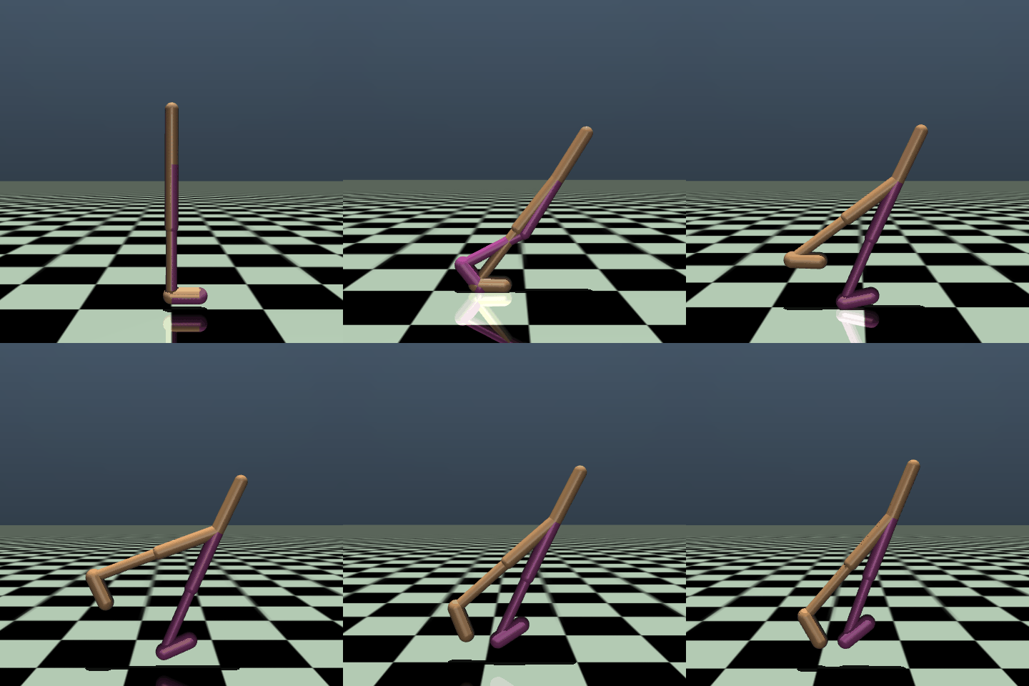Visual representation of the task. Image credits: Gymnasium

The results against three other baseline algorithms were:

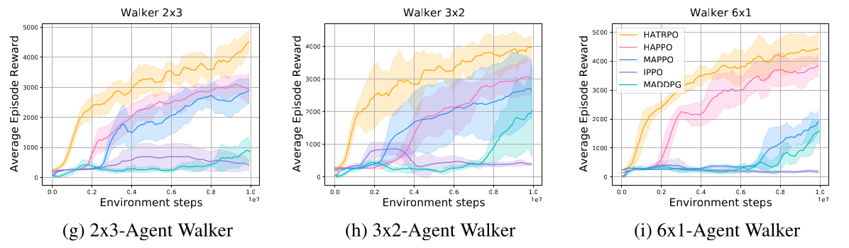Comparison between scenarios with 2, 3, and 6 agents, each controlling 3, 2, and 1 articulation, respectively.
Image obtained from Section 5 (Experiments and Results) of the original paper².

We can see that both algorithms present better results than the baselines, especially when the number of agents increases. It is also worth noting that the HATRPO presented better metrics than HAPPO. The authors argue that this happens since HATRPO implementation is closer to the original theoretical algorithm used to derive the monotonic improvement guarantee.

Bridging with the context of our project, just as the agents must learn together how to coordinate the different joints to walk, heterogeneous malware agents must learn how to cooperate to exploit a common target, and therefore they may use this exact sequential approach proposed in the paper.

Conclusion

Reinforcement Learning is a field currently undergoing significant development, which provides flexible models that suit the cybersecurity field well. The single-agent setting is already well consolidated with algorithms such as TRPO and PPO. This work extends both of them to the multi-agent scenario, while keeping the monotonic improvement guarantee.

Next steps

Based on the roadmap stated in the previous checkpoint, the next step is to reproduce the existing environment with the backdoored Reconfigurable Intelligent Surface (RIS) and establish the baselines for previous studies applying the PPO/HAPPO algorithms seen here to this context.

This post was made as a record of the progress of the research project “Learning to Exploit a Backdoored RL Controller: Coordinated MARL Attacks in Dynamic 6G Cyber-Physical Systems”, supervised by PhD candidate Alex Pierron and Professor Joaquin Garcia-Alfaro, in the IP Paris Master in Cybersecurity. Student supported by the France Excellence Eiffel scholarship, funded by the French Ministry for Europe and Foreign Affairs.

Stefano V. Albrecht, Filippos Christianos, and Lukas Schäfer. “Multi-Agent Reinforcement Learning: Foundations and Modern Approaches.” MIT Press, 2024. ↩︎ ↩︎²
Jakub Grudzien Kuba, Ruiqing Chen, Muning Wen, Ying Wen, Fanglei Sun, Jun Wang, and Yaodong Yang. “Trust Region Policy Optimisation in Multi-Agent Reinforcement Learning.” In International Conference on Learning Representations (ICLR), 2022, doi:10.48550/arXiv.2109.11251. ↩︎ ↩︎² ↩︎³
https://openai.com/index/hugging-face-incident-and-the-road-ahead/ ↩︎
John Schulman, Sergey Levine, Philipp Moritz, Michael I. Jordan, and Pieter Abbeel. “Trust Region Policy Optimization.” arXiv, 2015, doi:10.48550/arXiv.1502.05477.
A quick summary of it can be found in the OpenAI Spinning Up docs. ↩︎
John Schulman, Filip Wolski, Prafulla Dhariwal, Alec Radford, and Oleg Klimov. “Proximal policy optimization algorithms.” arXiv, 2017, doi:10.48550/arXiv.1707.06347.
A quick summary of it can be found in the OpenAI Spinning Up docs. ↩︎ ↩︎²
A policy space is $\eta$-soft if there exists $\eta \in \mathbb{R}$, with $0 < \eta \ll 1$, such that $\forall i \in \mathcal{N}$, $\forall \pi^i \in \Pi^i$, $\forall s \in \mathcal{S}$, and $\forall a^i \in \mathcal{A}^i$ we have $\pi^i(a^i \vert{} s) \ge \eta$. ↩︎
The order can be randomised at each iteration, which in fact is desirable, since it contributes to convergence, as demonstrated in ablation studies in Appendix F of the original article. ↩︎
Computing the true value for the advantage would require full knowledge of the environment dynamics, which is usually far from reality, and also would imply iterating over the full state-action space, usually unfeasible. ↩︎
Christian Schröder de Witt, Bei Peng, Pierre-Alexandre Kamienny, Philip H. S. Torr, Wendelin Böhmer, and Shimon Whiteson. “Deep Multi-Agent Reinforcement Learning for Decentralized Continuous Cooperative Control.” arXiv, 2020, doi:10.48550/arXiv.2003.06709v2. ↩︎

M2 Research Project

security ML RL

This post is licensed under CC BY 4.0 by the author.